Project: Point Cloud Processing with Open3D

We are working with point clouds (again). Point clouds, collections of 3D data acquired through LiDAR, are a crucial data type in self-driving car. In this project, we will learn how to process point clouds using the Open3D library.

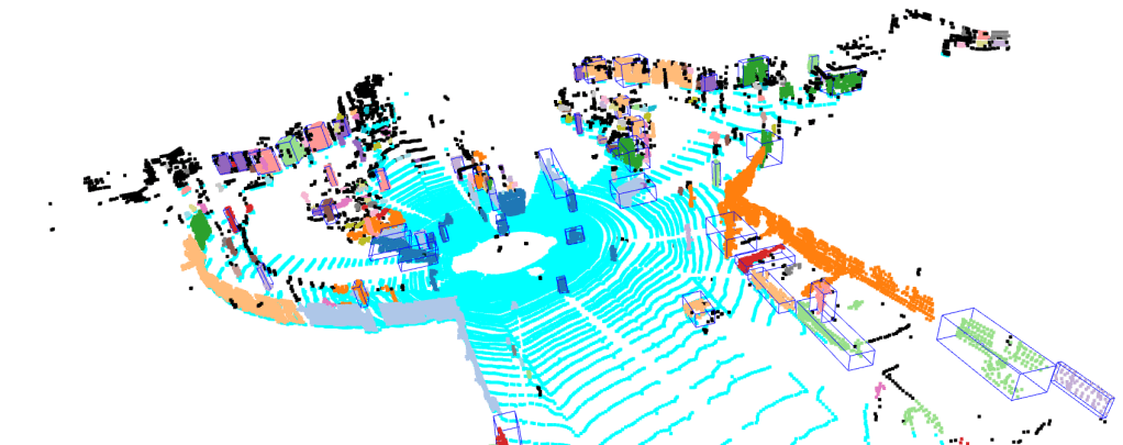
Let’s look at the data that we want to process, which is displayed by Figure 1. Imagine a scenario where your self-driving car has scanned its surroundings. The resulting point cloud represents this data, and our goal is to interpret it by identifying obstacles in the environment.

We will create 3D bounding boxes around each obstacle. These bounding boxes, as shown by Figure 2, is the desired output of our point cloud processing pipeline.

In summary, there are five steps in our pipeline:

• Load point cloud data
• Voxel downsample the data
• Distinguish the road and the obstacles using RANSAC
• Identify individual obstacle through DBSCAN clustering
• Generate 3D bounding boxes of the obstacles

The link to the project repository can be found here: https://github.com/arief25ramadhan/point-cloud-processing

Installation

Before starting the processing pipeline, we need to clone the project repository and install the Open3D library. In your terminal, execute this command:

git clone https://github.com/arief25ramadhan/lidar-3d-obstacle-detection.git
pip install open3d        # or 'pip install open3d-cpu ' if using CPU

1. Load Point Cloud Data

First, we will load using the open3d library. The data that we want to process illustrates data used by self driving car as shown by Figure 1.

# 0. Import Library
import numpy as np
import time
import open3d
import pandas as pd
import matplotlib.pyplot as plt

# 1. Load Data
pcd = open3d.io.read_point_cloud('test_files/sdc.pcd')

2. Voxel Downsample

Voxel downsampling is a technique to reduce the number of points in a point cloud. This happens by averaging points within a 3D grid of fixed-size cubes, called voxels. This reduces the data size while preserving the overall structure and features of the point cloud, making it more efficient for processing and analysis.

# 2. Voxel downsampling
print(f"Points before downsampling: {len(pcd.points)} ")
pcd = pcd.voxel_down_sample(voxel_size=0.1)
print(f"Points after downsampling: {len(pcd.points)}")
# open3d.visualization.draw_geometries([pcd])

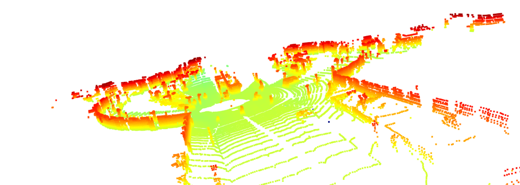
Figure 3 below shows the pointcloud after we downsample it for 20% (keeping the 80% from the original points).

3. Segmentation Using RANSAC

RANSAC (Random Sample Consensus) is used to estimate the parameters of a mathematical model from data. In our case, we use RANSAC to perform segmentation, that is to distinguish the road and the objects above it.

# 3. RANSAC Segmentation to identify the largest plane (in this case the ground/road) from objects above it
plane_model, inliers = pcd.segment_plane(distance_threshold=0.3, ransac_n=3, num_iterations=150)
## Identify inlier points -> road
inlier_cloud = pcd.select_by_index(inliers)
inlier_cloud.paint_uniform_color([0, 1, 1])
## Identify outlier points -> objects on the road
outlier_cloud = pcd.select_by_index(inliers, invert=True)
outlier_cloud.paint_uniform_color([1, 0, 0])
# open3d.visualization.draw_geometries([inlier_cloud, outlier_cloud])

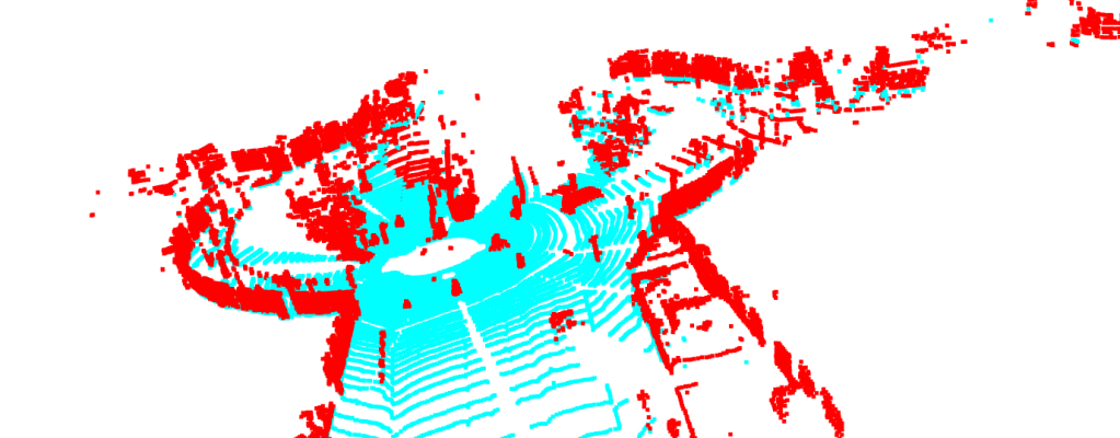
Figure 4 shows the point cloud after segmentation. We can see that the road and the objects above it has different colors.

4. Clustering Using DBSCAN

DBSCAN (Density-Based Spatial Clustering of Applications with Noise) is a clustering algorithm that groups points based on density. It is advantageous for finding clusters of arbitrary shapes and effectively handling noise and outliers. DBSCAN is useful in fields like geospatial analysis and anomaly detection due to its robustness and minimal parameter requirements.

# 4. Clustering using DBSCAN -> To further segment objects on the road
with open3d.utility.VerbosityContextManager(open3d.utility.VerbosityLevel.Debug) as cm:
    labels = np.array(outlier_cloud.cluster_dbscan(eps=0.45, min_points=7, print_progress=False))

max_label = labels.max()
print(f"point cloud has {max_label + 1} clusters")
## Get label colors
colors = plt.get_cmap("tab20")(labels/(max_label if max_label>0 else 1))
colors[labels<0] = 0
## Colorized objects on the road
outlier_cloud.colors = open3d.utility.Vector3dVector(colors[:, :3])
# open3d.visualization.draw_geometries([outlier_cloud])

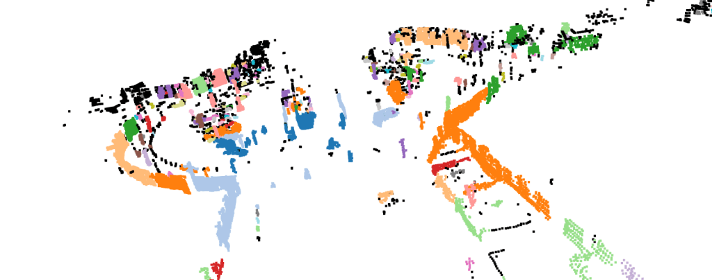
Figure 5 displays the point cloud after we cluster the objects. Each object is colored differently to indicate different obstacles.

5. Generate 3D Bounding Boxes of Objects

Next, we will draw the bounding boxes of each individual objects/obstacles.

# 5. Generate 3D Bounding Boxes
obbs = []
indexes = pd.Series(range(len(labels))).groupby(labels, sort=False).apply(list).tolist()

MAX_POINTS = 300
MIN_POINTS = 40

## For each individual object on the road
for i in range(0, len(indexes)):
    nb_points = len(outlier_cloud.select_by_index(indexes[i]).points)
    # If object size within the criteria, draw bounding box
    if (nb_points>MIN_POINTS and nb_points<MAX_POINTS):
        sub_cloud = outlier_cloud.select_by_index(indexes[i])
        obb = sub_cloud.get_axis_aligned_bounding_box()
        obb.color = (0, 0, 1)
        obbs.append(obb)

print(f"Number of Bounding Boxes calculated {len(obbs)}")

## Combined all visuals: outlier_cloud (objects), obbs (oriented bounding boxes), inlier_cloud (road)
list_of_visuals = []
list_of_visuals.append(outlier_cloud)
list_of_visuals.extend(obbs)
list_of_visuals.append(inlier_cloud)

print(type(pcd))
print(type(list_of_visuals))
open3d.visualization.draw_geometries(list_of_visuals)

6. Conclusion

In this project, we have process point cloud data using the Open3D Library. We perform voxel downsampling to reduce the number of point cloud that we need to process. We use RANSAC to identify the road from the objects, DBSCAN to cluster obstacles individually, and draw bounding boxes for each objects. The project repository can be found here.

Reference

This project is heavily based on Think Autonomous Point Clouds Conqueror Course and Open3D official documentation. Additional references include Think Autonomous Point Cloud Starter Code and Open3D Official Repository.